ESP32-P4 Deep Learning Tutorial: MNIST with PyTorch and ESP-DL
The topic of machine learning has fascinated me for several years, but my knowledge of it had remained fairly superficial. To truly understand how this fascinating technology works, I have now delved more deeply into the subject. My focus was specifically on Deep Learning, which is based on artificial neural networks with many layers.
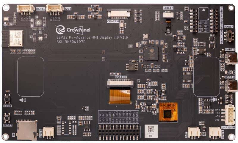
In this article I demonstrate the "Hello World" of machine learning: the automatic recognition of handwritten digits. This post is not an introduction to the fundamentals of artificial intelligence, as that field is far too extensive. Instead, I want to use a concrete example to walk through all the necessary steps – from training the neural network in Python (PyTorch), through quantization, all the way to the live deployment of the finished model. The model is trained on a PC and then run on an ESP32-P4 with a display. For this I use the CrowPanel Advance 7" ESP32-P4 HMI AI Display, which I recently reviewed.
The Software Stack: PyTorch and ESP-DL
A machine learning project for microcontrollers is, by its very nature, split into two parts: the computationally intensive training phase on the PC, and the execution phase (inference) on the chip.
PyTorch as Training Environment
For training I use PyTorch, one of the leading open-source deep learning frameworks. It enables fast computation of multidimensional matrices on the GPU and handles all the complex mathematics for adjusting the network weights automatically in the background.
On the data side, Dataset and DataLoader take care of shuffling, batching and parallel prefetching of training data. In this project they load the MNIST dataset together with custom handwritten digits, which are weighted 50-fold so that the few custom images do not get lost among the 60,000 MNIST samples.
ESP-DL and ESP-PPQ
The Espressif Deep Learning Framework (ESP-DL) provides optimized C++ libraries specifically developed to run neural networks efficiently on the ESP32-P4. On the hardware side, this software is massively accelerated on the ESP32-P4 (as well as the ESP32-S3) by the Processor Instruction Extensions (PIE). This instruction set extension uses the SIMD principle (Single Instruction Multiple Data) and processes data in a highly parallel manner via dedicated 128-bit wide vector registers, the so-called Q-registers of the processor.
The bridge between PyTorch (Python) and ESP-DL (C++) is ESP-PPQ (Post-Training Quantization). This framework takes the PyTorch model, compresses it from 32-bit floating-point numbers to 8-bit integers (Int8) and converts it into a .espdl file. Through this 8-bit quantization, exactly 16 parameters of the neural network fit simultaneously into a single 128-bit register of the ESP32-P4. The microcontroller can thereby execute 16 multiplications for the convolutional layers in a single instruction in parallel.
The Data Foundation: MNIST and Custom Images
The foundation of every machine learning project is the training data. For digit recognition there is the MNIST dataset, which contains 60,000 training images and 10,000 test images of handwritten digits. Each image is in 28x28 pixel grayscale format and shows a centered digit.
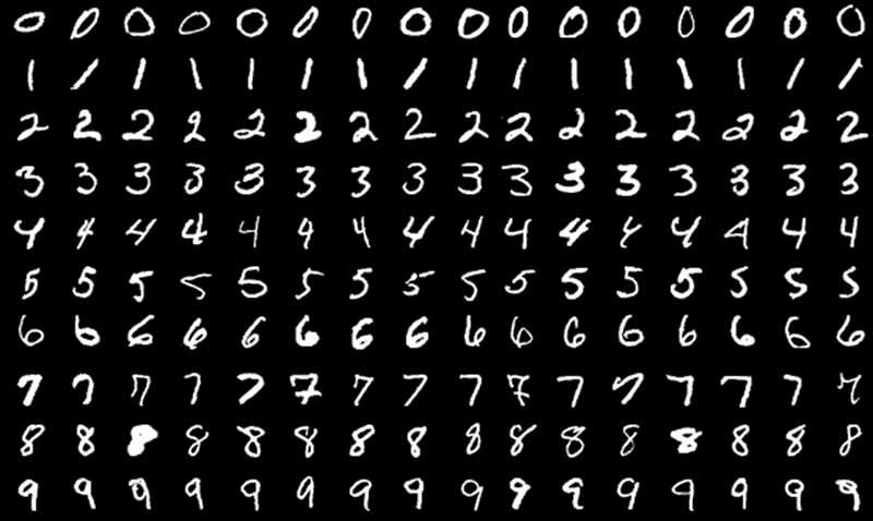
In principle, MNIST would be entirely sufficient for this simple demo, but the digits come predominantly from the American region, where there are some subtle differences from European digits. An American "1" is a single vertical stroke, while a European "1" has a distinctive upward stroke. An American "7" consists of two strokes, whereas the European variant has an additional horizontal bar in the middle. Due to this dataset bias, the neural network would interpret a typical European "1" with its upstroke as an American "7", leading to misclassifications.
I therefore collected as many handwriting samples as possible from friends using a tablet, and then used a Python script to automatically split the image into individual digits.
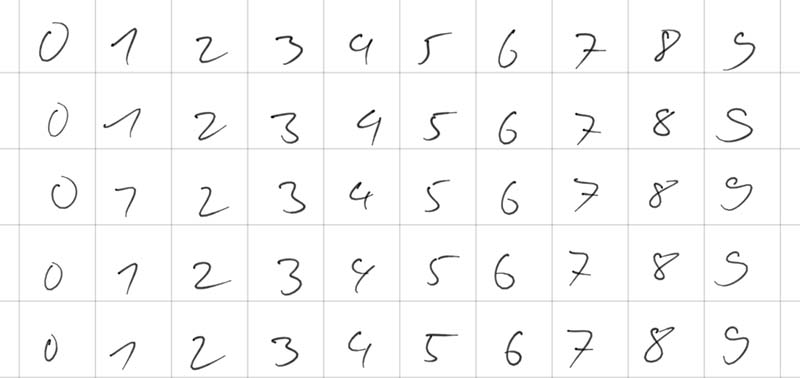
If these custom images were simply added to the 60,000 MNIST images, they would be completely lost in the large mass. Therefore a concept called oversampling (or dataset boosting) is applied. The images are duplicated in code when loaded into memory, so that they receive sufficient relevance during training.
In addition, the training data is artificially modified with each loading pass. This process is called data augmentation. Using the PyTorch library transforms, two random distortions are applied to each image:
- Random Rotation: The image is randomly rotated by up to 10 degrees left or right.
- Random Affine (Translation): The image is randomly shifted by up to 10 percent along the X or Y axis.
Through this "wobbling and shifting", the network sees a slightly altered version of the same digit in each training epoch. This forces the model to learn the fundamental shape of the digit rather than relying on exact pixel coordinates.
The last very important preprocessing step is normalization. Grayscale images normally consist of pixel values between 0 and 255. In PyTorch these are first converted into tensors with values between 0.0 and 1.0. However, artificial neural networks train fastest and most stably when the input data is centered around zero. Therefore the operation Normalize((0.1307,), (0.3081,)) is applied, which represents the global mean (0.1307) and standard deviation (0.3081) of the entire MNIST dataset.
The Architecture of the Convolutional Neural Network
Convolutional Neural Networks are frequently used in image recognition. I have therefore also opted for this network type in this project. Since this network later needs to run on an ESP32-P4, it is designed very simply and largely follows the examples commonly found for the MNIST dataset.
Since it is the central part of the entire project, I would like to go into the individual layers in a bit more detail here. The CNN is conceptually divided into two main phases:
- Feature Extraction: Two convolutional blocks that progressively extract abstract image features, from simple edges to complex curves.
- Classification Head: Two fully connected layers that derive from these extracted features which digit it is.
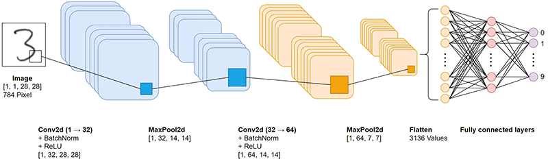
An image exists in memory as a multidimensional matrix (tensor). The input via the touch display provides the network with a tensor of dimension [1, 1, 28, 28]:
- 1 image (the batch size; during inference on the microcontroller only a single image is ever processed).
- 1 color channel (grayscale; RGB color information is not needed).
- 28 pixels height.
- 28 pixels width.
Each of the 784 pixels (28×28) has a floating-point value. Through the upstream normalization in the Python script, these values are centered around zero (e.g. between -1.0 and +1.0). These 784 values form the information basis for the model.
Low-Level Feature Extraction
The Convolution (Conv2d)
self.conv1 = nn.Conv2d(1, 32, kernel_size=3, padding=1)
Convolution forms the foundation of feature extraction. A 3x3 pixel filter (the kernel) slides step by step across the entire image. At each position, the values of the filter are multiplied with the underlying image pixels and summed up.
The crucial point is that the values within these filters are not pre-programmed but are learned through the training process. The parameter out_channels=32 defines that the network learns 32 different filters in parallel. Each filter specializes in a specific feature, for example vertical edges or diagonal lines.
- kernel_size=3: A 3x3 filter represents an established standard in image processing. It is large enough for pattern recognition, yet small enough for high computational efficiency.
- padding=1: Without padding the image would shrink after the convolution (from 28x28 to 26x26). The padding adds an invisible border of zeros around the image so that the output remains at exactly 28x28 pixels. Information loss at the edges is thus avoided.
The number of parameters in this layer is calculated as follows: 1 (input channel) × 32 (filters) × 3 × 3 (kernel size) + 32 (bias values) = 320 parameters.
Batch Normalization (BatchNorm2d)
self.bn1 = nn.BatchNorm2d(32)
When data flows through deep networks, the phenomenon of internal covariate shift often arises. After a weight update in the first layer, the value distribution changes drastically, destabilizing the subsequent layers.
Batch Normalization solves this problem by centering and scaling the activations of each of the 32 channels. The training process is thereby considerably stabilized and convergence is accelerated.
The Activation Function: ReLU
x = F.relu(x)
Nach der Faltung durchlaufen die Werte die ReLU-Funktion (Rectified Linear Unit): f(x)=max(0,x)
Negative Werte werden auf Null gesetzt, positive Werte bleiben erhalten. Diese nicht-lineare Transformation ist zwingend erforderlich. Ein Netz ohne Nicht-Linearität lässt sich mathematisch auf eine einzige lineare Gleichung reduzieren und könnte keine komplexen, nicht-linearen Entscheidungsgrenzen erlernen.
After the convolution, the values pass through the ReLU function (Rectified Linear Unit): f(x) = max(0, x). Negative values are set to zero, positive values are retained. This non-linear transformation is strictly necessary. A network without non-linearity can be mathematically reduced to a single linear equation and would be unable to learn complex, non-linear decision boundaries.
Dimensionality Reduction: MaxPooling
self.pool = nn.MaxPool2d(2, 2)
x = self.pool(x)
A 2x2 pixel window slides with a stride of 2 across the 32 feature maps. Only the maximum value is retained; all other values are discarded.
This halves the spatial resolution from 28x28 to 14x14 pixels and offers two advantages:
- Computational load: The data volume for the subsequent layers is reduced by 75%.
- Translation invariance: Small spatial shifts of a feature no longer matter. Max pooling absorbs these variations, making the network more robust to handwriting differences.
High-Level Feature Extraction
The second block operates on the same principles, but processes data at a higher level of abstraction. The input consists no longer of raw pixels but of the 32 feature maps from Block 1.
The number of filters is doubled to 64. At this level, the network combines the simple edges from the first block into more complex constructs such as arcs, intersections or loops. Since the number of possible combinations is higher, more filters are needed.
The number of parameters in this layer: 32 (in) × 64 (out) × 3 × 3 (kernel) + 64 (bias) = 18,496 parameters. After passing through this block and a further max pooling step, the resolution has shrunk to 7x7 pixels. The result is 64 highly concentrated, semantic matrices.
Flattening & Dropout
x = x.view(-1, 64 * 7 * 7)
self.dropout = nn.Dropout(0.5)
Flattening
The final classification layers require a flat, one-dimensional vector. Using the view function, the 64 maps of 7x7 pixels each are transformed into a continuous vector: 64 × 7 × 7 = 3,136 values. The image has thus been translated into a numerical "fingerprint" of 3,136 features.
Dropout
A well-known problem in deep neural networks is overfitting, the undesirable memorization of the exact training data instead of the underlying patterns. To prevent this, dropout is employed. During training, 50% (p=0.5) of connections are randomly deactivated at each forward pass. This forces the architecture to build robust redundancies and prevents co-adaptation of individual neurons. During inference, dropout is fully deactivated.
Classification Head
self.fc1 = nn.Linear(64 * 7 * 7, 128)
self.fc2 = nn.Linear(128, 10)
The fully connected (dense) layers handle the final classification. The layer fc1 connects each of the 3,136 features to 128 new neurons. Parameter count: 3136 × 128 + 128 = 401,536 parameters. More than 90% of all model parameters reside in this single matrix multiplication. These 128 neurons aggregate the information and learn which geometric combinations are characteristic for which digits.
After a final ReLU activation, fc2 reduces these 128 signals to exactly 10 output values (logits) for the digits 0 through 9.
In total, the model comprises approximately 421,642 trainable parameters. Quite a high number for such a simple task, at least until one realizes that current language models now have over a trillion parameters.
Training: Implementation in PyTorch
Training is typically divided into two separate functions: the training loop and the validation loop.
The Training Cycle (Forward and Backward Pass)
The train function is the heart of machine learning. Here the more than 420,000 parameters of the network adapt iteratively to correctly identify digits.
First, the PyTorch model is set to training mode with model.train(). Dropout now begins randomly severing connections, and BatchNorm computes the mean values for the current batch. The train_loader is then iterated, loading images in batches (e.g. 64 images at a time) onto the processor or graphics card. The actual learning step in the loop consists of four fundamental operations:
optimizer.zero_grad()(Reset): Before new computations are made, the old gradients from the previous pass must be reset to zero. Otherwise PyTorch would continuously accumulate them, which would immediately destroy the training.output = model(data)(Forward Pass): The 64 input images flow through the network. The result is 64 vectors with 10 raw output values (logits) each.loss = F.cross_entropy(...)(Loss Calculation): Here the network's prediction is compared with the actual label (the true digit). The cross-entropy loss function is the mathematical gold standard for classification problems. It penalizes the model particularly harshly when it is extremely confident about a wrong prediction.loss.backward()andoptimizer.step()(Learning): Through backpropagation, PyTorch calculates how strongly each individual parameter in the network contributed to the measured error. The optimizer (in this project the Adam optimizer) takes this information and adjusts the weights minimally to reduce the error in the next pass. This process corresponds to iterative gradient descent.
Validation
To verify that the model is genuinely learning the digits and not just memorizing them (overfitting), the test function is called after each training epoch. It uses a separate test_loader containing 10,000 images the network has never seen before.
Here the model is switched to inference mode with model.eval(). Dropout is deactivated so that 100% of neurons are now active. BatchNorm therefore falls back on the learned global average values. Since no weights are adjusted during the test phase, computation is disabled with with with torch.no_grad().
The console output shows the progression of the learning process. Already by epoch 5 the model exceeds the 99% mark on the unseen test images:
Train Epoche: 1 [...]    Loss: 0.177625
Test set: Average loss: 0.0673, Accuracy: 9760/10000 (97.60%)
...
Train Epoche: 5 [...]    Loss: 0.123470
Test set: Average loss: 0.0327, Accuracy: 9901/10000 (99.01%)
...
Train Epoche: 29 [...]   Loss: 0.069147
Test set: Average loss: 0.0177, Accuracy: 9946/10000 (99.46%)
This output is also very useful for detecting overfitting. If the loss of the training loop were to continue falling steadily towards 0 while the average loss of the test loop suddenly starts rising again, the model would be beginning to simply memorize the training data.
In this training run, however, that is not the case. The test data loss stabilizes at a very low level without rising again significantly. This proves that the implemented countermeasures – in particular dropout and the dynamic data augmentation through shifting and rotating the images – work perfectly and that the model generalizes robustly. The model reaches its best performance in epoch 29 with an accuracy of 99.46%.
Quantization: Preparing the Model for the ESP32-P4
The trained PyTorch model works with 32-bit floating-point numbers. For the ESP32-P4 to use this model, the model parameters must be converted to 8-bit or 16-bit integers. For a simple MNIST model, the compact Int8 format is entirely sufficient. This allows the hardware accelerator of the ESP32-P4 to process 16 Int8 values in a single instruction in parallel via the SIMD principle, massively accelerating inference.
The ONNX Export
First, the model is converted to ONNX format via a dummy input tensor. ONNX (Open Neural Network Exchange) is an open format developed by Microsoft, Meta and AWS that allows the exchange of deep learning and machine learning models between different frameworks. The parameter do_constant_folding=True is important here. It integrates static computations such as batch normalization directly into the convolutional weights. This frees the network from superfluous computation nodes and noticeably accelerates later execution on the microcontroller.
Calibration and Quantization with esp_ppq
The conversion from 32-bit floating-point numbers to 8-bit integers is handled by the Post-Training Quantization framework from Espressif (esp_ppq). To determine the optimal scaling, the quantizer performs a calibration step. For this, 32 real images from the test dataset are passed to the API.
Using the ONNX model and these calibration images, the function quantize_onnx_model generates the quantized network for the target architecture TargetPlatform.ESPDL_INT8. Finally, `export_ppq_graph` produces the finished .espdl file that the ESP32-P4 can process.
Deployment on the ESP32-P4: Inference in C++
In the last step, the trained and quantized model is executed on the microcontroller. As the target platform I use the CrowPanel Advance 7" ESP32-P4 HMI AI Display. This board provides both the necessary computing power and a good touch panel for digit input.
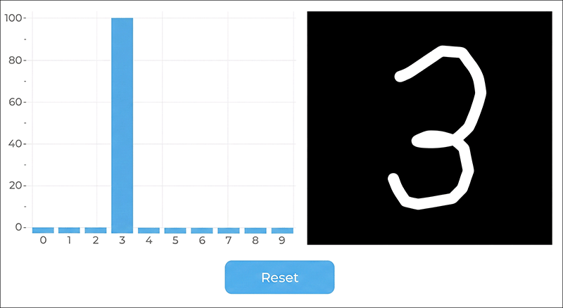
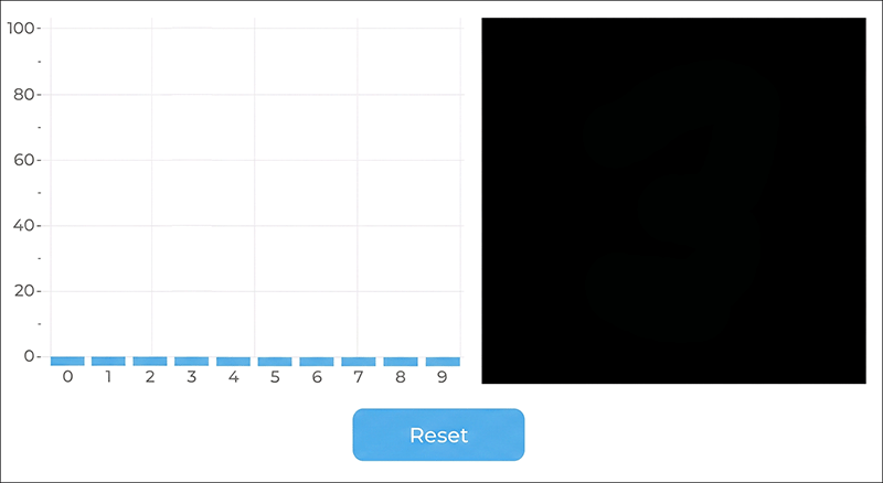
To test the model live, I developed a simple application. As soon as one starts drawing a digit on the panel, the network computes the probability values in real time and displays them directly as a bar chart.
Software Structure and User Interface
I created the user interface with EEZ-Studio. It consists of only three parts: the bar chart, a canvas for drawing, and the reset button.
The overall project structure is as follows:
ESP32-MNIST-Demo/
│
├── build/
│
├── eez-studio/                       (EEZ Studio Project)
│
├── main/
│   ├── display/                      (MIPI DSI Display)
│   │   ├── display.c
│   │   └── display.h
│   ├── gui/                          (LVGL Canvas & Chart)
│   │   ├── canvas_paint.c
│   │   ├── canvas_paint.h
│   │   ├── chart_display.c
│   │   └── chart_display.h
│   ├── mnist/                        (Model Inference Code)
│   │   ├── mnist_inference.cpp
│   │   ├── mnist_inference.h
│   │   ├── mnist_task.c
│   │   └── mnist_task.h
│   ├── ui/                           (EEZ-Studio generated Code)
│   │   ├── actions.h
│   │   ├── fonts.h
│   │   ├── images.c
│   │   ├── images.h
│   │   ├── screens.c
│   │   ├── screens.h
│   │   ├── structs.h
│   │   ├── styles.c
│   │   ├── styles.h
│   │   ├── ui.c
│   │   ├── ui.h
│   │   └── vars.h
│   ├── CMakeLists.txt
│   ├── idf_component.yml
│   └── main.c
│
├── managed_components/               (Used Components)
│   ├── espressif__cmake_utilities/
│   ├── espressif__dl_fft/
│   ├── espressif__esp-dl/
│   ├── espressif__esp-dsp/
│   ├── espressif__esp_lcd_ek79007/
│   ├── espressif__esp_lcd_touch/
│   ├── espressif__esp_lcd_touch_gt911/
│   ├── espressif__esp_lvgl_port/
│   ├── espressif__esp_new_jpeg/
│   └── lvgl__lvgl/
│
└── spiffs/                            (PyTorch generated Model)
    └── mnist_advanced_cnn.espdl
The project was created with Visual Studio Code and the ESP-IDF plugin from Espressif.
The Model in Flash Memory: SPIFFS and Partitions
For the microcontroller to load the neural network, the generated ESPDL file is placed in a folder called spiffs within the ESP32 project. When the project is uploaded via the ESP-IDF plugin, the contents are written directly into the flash memory of the ESP32-P4. For this, the file partitions.csv must be adjusted to allocate sufficient storage space (at least the size of the model file) to the SPIFFS filesystem:
# ESP-IDF Partition Table
# Name,   Type, SubType, Offset,  Size, Flags
# Note: if you have increased the bootloader size, make sure to update the offsets to avoid overlap

nvs,      data, nvs,     ,        0x4000,
otadata,  data, ota,     ,        0x2000,
phy_init, data, phy,     ,        0x1000,
factory,  app,  factory,  ,       0x3F0000,
ota_0,    app,  ota_0,   ,        0x3F0000,
ota_1,    app,  ota_1,   ,        0x3F0000,
model,    data, spiffs,  ,        0x3F0000,
At system startup, this filesystem is mounted in C++ code and the model is loaded directly into RAM via the dl::Model class:
bool mnist_inference_init(void)
{
    /* Mount SPIFFS with model file */
    esp_vfs_spiffs_conf_t spiffs_conf = {
        .base_path = "/model",
        .partition_label = "model",
        .max_files = 2,
        .format_if_mount_failed = false,
    };
    esp_err_t ret = esp_vfs_spiffs_register(&spiffs_conf);
    if (ret != ESP_OK) {
        ESP_LOGE(TAG, "SPIFFS mount failed: %s", esp_err_to_name(ret));
        return false;
    }

    /* Load model */
    ESP_LOGI(TAG, "Loading model...");
    model = new dl::Model("/model/mnist_advanced_cnn.espdl",
                          fbs::MODEL_LOCATION_IN_SDCARD);
    ESP_LOGI(TAG, "Model loaded.");

    return true;
}
Besides SPIFFS, ESP-DL also supports loading the model from an SD card or embedding it directly into the application binary.
Hardware-Accelerated Scaling with the PPA
The neural network expects exactly the format of the training data, a 28x28 pixel grayscale image. The display, however, has a resolution of 1024x600 pixels and the drawing canvas has a size of 448x448 pixels. This size is deliberately chosen because 448 can be divided by 16 without rounding errors (28 times 16 = 448).
If the microcontroller were to downscale this large image in software at every touch input, noticeable delays while drawing would result. This is where the integrated Pixel Processing Accelerator (PPA) of the ESP32-P4 comes into play. Via the SRM block (Scale, Rotate, Mirror) of the PPA, the 448x448 RGB image is scaled down entirely in hardware by a factor of 1/16:
const uint8_t *ppa_resize(void)
{
    ppa_srm_oper_config_t srm_cfg = {
        .in = {
            .buffer     = canvas_buf,
            .pic_w      = CANVAS_WIDTH,
            .pic_h      = CANVAS_HEIGHT,
            .block_w    = CANVAS_WIDTH,
            .block_h    = CANVAS_HEIGHT,
            .block_offset_x = 0,
            .block_offset_y = 0,
            .srm_cm     = PPA_SRM_COLOR_MODE_RGB565,
        },
        .out = {
            .buffer      = srm_out_buf,
            .buffer_size = srm_out_buf_size,
            .pic_w       = PPA_OUT_SIZE,
            .pic_h       = PPA_OUT_SIZE,
            .block_offset_x = 0,
            .block_offset_y = 0,
            .srm_cm      = PPA_SRM_COLOR_MODE_RGB565,
        },
        .rotation_angle = PPA_SRM_ROTATION_ANGLE_0,
        .scale_x        = PPA_SCALE_FACTOR,
        .scale_y        = PPA_SCALE_FACTOR,
        .mode           = PPA_TRANS_MODE_BLOCKING,
    };

    esp_err_t ret = ppa_do_scale_rotate_mirror(ppa_srm_handle, &srm_cfg);
    if (ret != ESP_OK) {
        ESP_LOGE(TAG, "PPA SRM failed: %s", esp_err_to_name(ret));
        memset(gray_buf, 0, sizeof(gray_buf));
        return gray_buf;
    }

    // ... Convert RGB565 to grayscale ...

    return gray_buf;
}
The microcontroller is thus considerably relieved and only needs to convert the 28x28 pixel image to grayscale.
Inference, Normalization and Quantization Mathematics
Before these grayscale images are processed by the neural network, they must be normalized in exactly the same way as in the Python training script (mean 0.1307 and standard deviation 0.3081). Since the model exists as an 8-bit integer network, the ESP-DL library provides the scaling exponent calculated during calibration via input->get_exponent(). The normalized floating-point numbers are multiplied by this exponent, rounded and clamped to the valid Int8 range (-128 to 127).
Once the image data has been written into the input tensor, a single call to model->run() suffices. Thanks to the PIE vector instructions, this inference process takes only about 20 milliseconds. The raw Int8 output values (logits) are then converted back to floating-point numbers:
bool mnist_inference_run(const uint8_t *gray_28x28, float scores[MNIST_NUM_CLASSES])
{
    if (!model) return false;

    dl::TensorBase *input = model->get_input();
    dl::dtype_t input_dtype = input->get_dtype();
    int input_exponent = input->get_exponent();

    /* Int8 model: normalize then quantize with model's exponent */
    float scale = powf(2.0f, (float)(-input_exponent));
    int8_t *dst = (int8_t *)input->get_element_ptr();
    for (int i = 0; i < 28 * 28; i++) {
        float pixel = gray_28x28[i] / 255.0f;
        float normalized = (pixel - MNIST_MEAN) / MNIST_STD;
        float quantized = roundf(normalized * scale);
        if (quantized > 127.0f) quantized = 127.0f;
        if (quantized < -128.0f) quantized = -128.0f;
        dst[i] = (int8_t)quantized;
    }

    /* Run inference */
    model->run();

    /* Read output scores */
    dl::TensorBase *output = model->get_output();
    int output_exponent = output->get_exponent();
    dl::dtype_t output_dtype = output->get_dtype();
    int num = output->get_size();
    if (num > MNIST_NUM_CLASSES) num = MNIST_NUM_CLASSES;

    for (int i = 0; i < num; i++) {
        int8_t raw = output->get_element<int8_t>(i);
        scores[i] = (float)raw * powf(2.0f, (float)output_exponent);
    }

    return true;
}
The file chart_display.c offers two visualization modes for the display, selectable via the constant CHART_MODE_RAW.
The first variant uses a softmax function to convert the network outputs into probabilities. Through the exponential calculation, the highest individual value is strongly amplified while the remaining outputs can drop to near zero. The focus here is on making a clear decision for a single digit.
The second variant uses direct scaling of the output values. In this mode, the original relations of the prediction are preserved and the bars show the actual weighting relative to each other. With this method one can clearly see how confident or uncertain the network's values are.
Live Demo: The System in Action
How smoothly the ESP-DL neural network runs with the ESP32-P4 is shown in the short demo video below. The output uses direct scaling.
I could spend hours playing with the display, because it is absolutely fascinating to watch the artificial intelligence at work. I find it particularly interesting how often just a single stroke is enough to make the network change its mind, so that the probability suddenly jumps from one digit to another.
However, a few quirks become apparent during testing. When using the softmax variant, one digit almost always shows 100% probability, even when no digit has clearly been drawn. This behavior is not a model error but a purely visual phenomenon of this particular function. Switching to direct scaling of the output values, the system behaves as expected and correctly shows a low value for all digits when given nonsensical input.
The second quirk concerns positioning on the drawing canvas. For a reliable prediction, the digit must be drawn centered and relatively large. The reason for this lies in the structure of the training data used. In the original MNIST dataset, all digits are precisely aligned in the center of the image and fill the available space almost completely. If one draws a small number in an outer corner of the touch display, the digit will usually not be recognized.
Conclusion
I worked on this project for quite a long time until the system was running without errors. But the effort was worth it, because I learned a lot during the development process. In practice, you understand such concepts much better than through pure theory from books. I also have ideas for useful applications at home, but at the moment I simply don't have a source for the appropriate training data. In the end, every deep learning project stands or falls on this data basis. The Python and C++ code for the entire project is available for you to try out on GitHub.